はじめに
LoGフィルタを用いた画像のエッジ検出方法について解説します。SciPyのndimageモジュールに含まれるgaussian_laplace関数を活用すると、ガウシアンフィルタとラプラシアンフィルタを組み合わせたLoG(Laplacian of Gaussian)フィルタを簡単に実装できます。
このフィルタは、画像の急激な輝度変化(エッジ)を検出するのに優れており、ノイズに強いという特徴があります。本記事では、実際のコード例とともに、パラメータの調整方法や処理結果の可視化についても詳しく説明していきます。
LoGフィルタの基本概念
LoG(Laplacian of Gaussian)フィルタは、画像処理における重要なエッジ検出手法の一つです。このフィルタは以下の二つの処理を組み合わせています:
- ガウシアンフィルタ処理:まず画像にガウシアンフィルタを適用してノイズを低減します。
- ラプラシアン演算:次に、平滑化された画像に対してラプラシアン演算を行い、輝度の急激な変化(エッジ)を検出します。
この二段階の処理を一度に行えるのがLoGフィルタの特徴であり、SciPyのndimage.gaussian_laplace関数を使用することで簡単に実装できます。
コード&解説
モジュールのインポート
バージョン
画像の読み込み
下記サイトから画像を取得し、plt.imread()で読み込みます。

グレースケール変換
skimage.colorモジュールのrgb2gray関数を使用して、RGB画像をグレースケール画像に変換します。変換した画像をcmap=”bone”パラメータで表示すると、以下のような結果になります。
LoGフィルタ
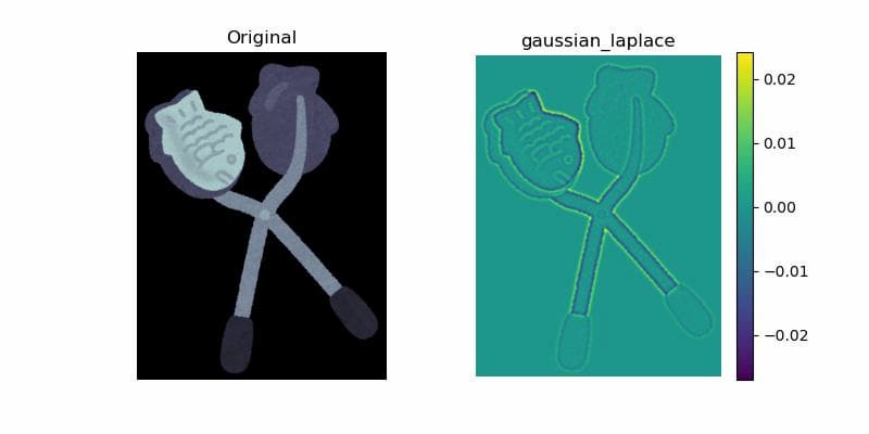
gaussian_laplaceをsigma=3に設定したLoGフィルタを適用すると、以下のような結果が得られます。
LoGフィルタを使用する際の重要なパラメータはsigma(標準偏差)です。このパラメータによって検出されるエッジの特性が変わります:
- 小さい値のsigma:細かいエッジを検出しますが、ノイズの影響を受けやすくなります。
- 大きい値のsigma:大まかなエッジのみを検出し、細部の情報は失われますが、ノイズに強くなります。
最適なsigma値は対象画像や目的によって異なるため、いくつかの値を試して最適な結果を得ることが重要です。
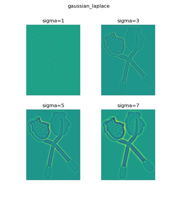
LoGフィルタのsigmaを変えた場合
ガウス微分フィルタのsigmaを変えた時の変化は以下のようになります。
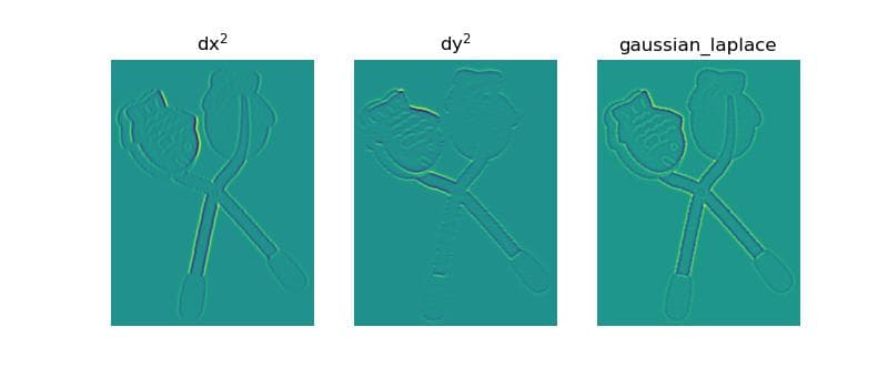
手動でLoGフィルタ
LoGフィルタはガウス関数の2階微分フィルタであるため、x方向の結果はndi.gaussian_filter(img_g, (sigma,sigma), (0,2))で得られます。y方向の結果はorderを(2,0)とした場合に得られます。エッジの強度画像は、これらの各成分の和として計算できます。
まとめ
SciPyのndimage.gaussian_laplace関数を使用したLoGフィルタは、画像のエッジを効果的に検出するための強力なツールです。適切なパラメータ設定と前処理を行うことで、様々な画像処理タスクに応用できます。実際の応用では、対象画像の特性に合わせてsigma値を調整し、必要に応じて閾値処理などの後処理を組み合わせることで、より精度の高い結果を得ることができます。
参考


コメント