はじめに
この記事では、scikit-imageライブラリのskimage.measure.find_contours関数を使用して、バイナリ画像から対象物の輪郭を検出し、画像上に表示する方法について説明します。画像処理において輪郭検出は物体認識や形状分析に重要な技術です。
コード
解説
モジュールのインポートなど
画像の生成
最初にnp.zeros((s, s))を使用して256×256のゼロ行列を生成します。次に、(s*np.random.random((2, n**2))).astype(int)で0〜255の範囲のランダムな整数を(2,36)の形状で生成します。そして、生成した座標点[points[0], points[1]]に対応する画像im上の要素を1に設定し、ndimage.gaussian_filterを適用してぼかすことで最終的な画像データを作成しました。
大津の方法(threshold_otsu)を使用してしきい値を取得します。このしきい値で画像を二値化し、clear_border関数で画像境界に接している部分を除去します。
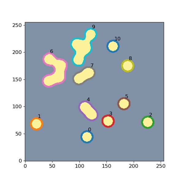
輪郭を検出
find_contours関数を使用して輪郭を検出します。バイナリ画像の場合、検出に用いる閾値は0と1の中間値である0.5を設定します。
結果の表示
figを作成した後、contours内に格納されている輪郭データをenumerateを使って一つずつプロットします。データの開始点の座標にax.text()でインデックスを表示し、ax.imshowで画像を表示することで、輪郭線が描画された画像が得られます。
find_contoursの値を変えたときの変化
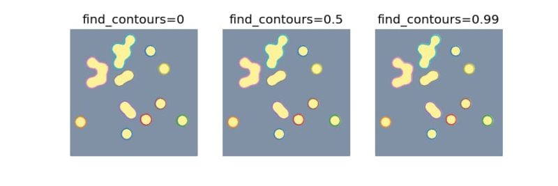
図の左から順に、find_contoursの閾値を0、0.5、0.99と変化させた結果を示しています。見た目には大きな変化が見られませんが、各閾値で得られる輪郭データの配列の形状を比較すると以下のような違いがあります。
閾値0でfind_contoursを実行したcontours0は他と比較して要素数が少ないことが分かります。また、閾値0.99と0.5でfind_contoursを実行したcontours1とcontours05の差を取ると、値が僅かに異なっていることが確認できます。
まとめ
scikit-imageのfind_contours関数は、バイナリ画像から対象物の輪郭を簡単に検出するための強力なツールです。この関数を使用することで、画像内の対象物の形状を分析したり、物体認識のための前処理を行ったりすることができます。
輪郭検出は画像処理のパイプラインにおいて重要なステップであり、物体の形状や位置に関する貴重な情報を提供します。scikit-imageを使えば、わずか数行のコードで効果的な輪郭検出を実装することができます。
参考


コメント