はじめに
scikit-learnのk-means法(KMeans)を使用したクラスタリング手法について解説します。この記事では、sklearn.datasets.make_blobsで生成したデータに対してクラスタリングを行う方法を学びます。
解説
モジュールのインポートなど
バージョン
データの生成
make_blobsを使用してデータを生成します。make_blobsの詳細については下記記事で解説しています。
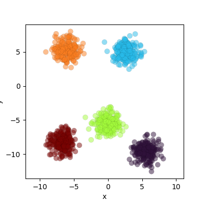
データの塊の数を5に設定し、データのばらつき(標準偏差)を示すcluster_stdパラメータを1、再現性のためのrandom_stateを10に指定しました。生成したデータを表示すると以下のようになります。
クラスター数
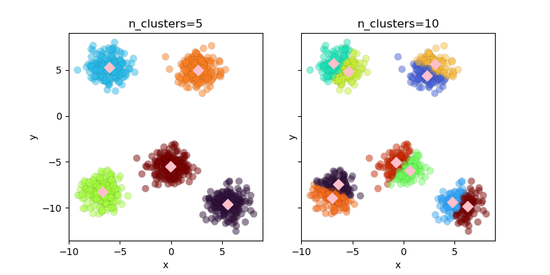
k-means法では自分でクラスター数を決める必要があります。ここでは、クラスター数を5と10に設定した場合の結果を示します。
KMeans(n_clusters)でモデルを設定します。設定したモデルに.fit(X)を適用することでクラスタリングを実行し、フィットした結果の.labels_属性からクラスターのラベルを取得できます。
結果の表示
cluster_centers_属性を使用することで、クラスタリング後に収束した各クラスタの重心座標を取得できます。
初期値
クラスターの中心の初期値はinitパラメータで変更できます。デフォルトは”k-means++”で、これにより適切な位置に初期値が設定されます。”random”を指定すると、ランダムに初期値が決定されます。n_initは初期値を設定する試行回数、max_iterは最適化計算の最大繰り返し回数です。ここでは両方とも1に設定して初期値の位置を確認します。
結果の表示
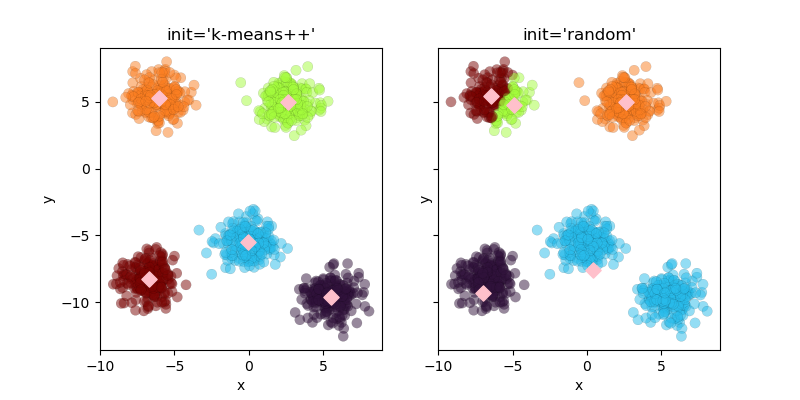
初期値がk-means++の場合、計算回数1回でも効果的なクラスタリングが実現できます。一方、randomオプションを使用すると初期値がランダムに設定されるため、1回の計算ではクラスタリング精度が低下することが明らかです。
収束の判断パラメータ tol
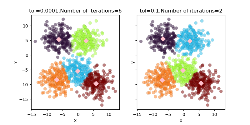
計算は誤差がtolの値を下回った時点で終了します。以下では、tol=0.1とtol=0.0001の場合のクラスタリング結果を比較します。
結果の表示
.n_iter_属性を使用することで計算の反復回数を確認できます。tolが0.0001の場合は6回、tolが0.1の場合は2回の計算で収束しています。
まとめ
k-means法は比較的シンプルながら強力なクラスタリング手法です。scikit-learnのKMeansクラスを使うことで、簡単に実装できることが分かりました。クラスタ数の決定にはエルボー法やシルエット分析が有効で、適切なパラメータ設定により精度の高いクラスタリングが可能です。
参考


コメント