はじめに
j今回はJupyter Notebookで画像分析を対話的に行う方法について解説します。具体的には、ipywidgetsのIntSliderとscikit-imageのprofile_line関数を組み合わせて、画像上の任意の位置における強度プロファイルをリアルタイムで取得・表示する方法を紹介します。
なお、profile_lineについては下記記事で解説しました。
[scikit-image] 71. 画像の強度プロファイルを任意の範囲で表示(skimage.measure profile_line)
scikit-imageのprofile_line関数を使用して、画像上の任意の2点間の強度プロファイル(輝度変化)を可視化する方法について解説します。画像処理における信号強度の分析や特徴抽出に役立つ手法です。
sabopy.com
2020.03.04
コード
解説
モジュールのインポートなど
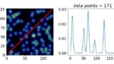
画像データの作成
用いる画像については、下記記事と同様に作成しました。
[matplotlib] 57. imshow使用時に軸を画像から離して表示する方法
matplotlibのplt.imshowで画像表示する際に軸を画像から離して配置する方法を解説します。tick_paramsとspinesの設定で軸の位置を調整し、視認性を高めるテクニックを紹介します。
sabopy.com
2020.01.23
画像の表示
make_axes_locatableを使用してカラーバーを画像の上に配置し、cax.xaxis.set_ticks_position(‘top’)を適用することでカラーバーの目盛りを上部に表示しました。
ipywidgetsの設定
plotの作成
まず、空のプロットを作成して、widgetsから取得した値を表示できるようにします。このプロットは、skimageのprofile_line関数で取得した強度プロファイルデータを表示するためのもので、画像の横(ax[1])に配置されます。
IntSliderの作成
IntSliderを使用して、プロファイルの開始点と終了点の座標を取得します。
Sliderの値を変えたときに行う処理
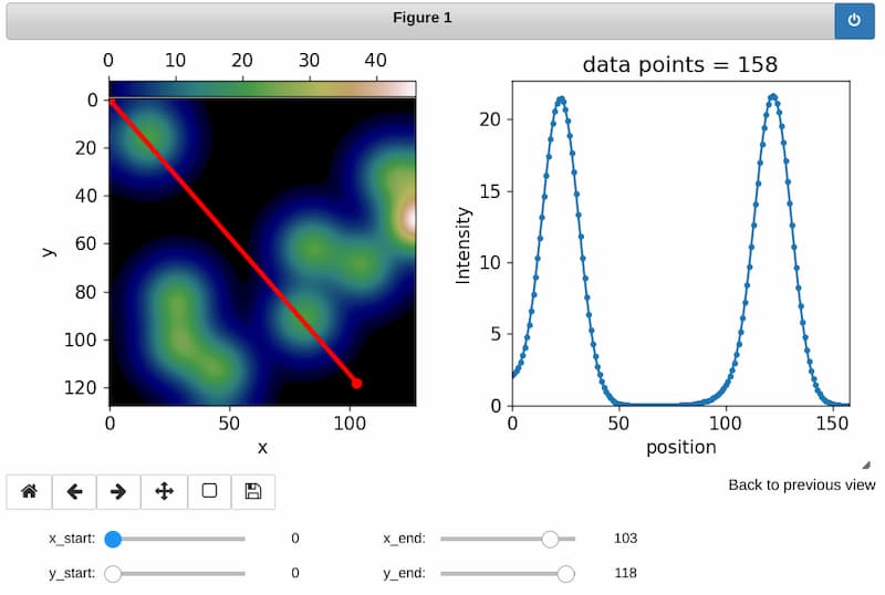
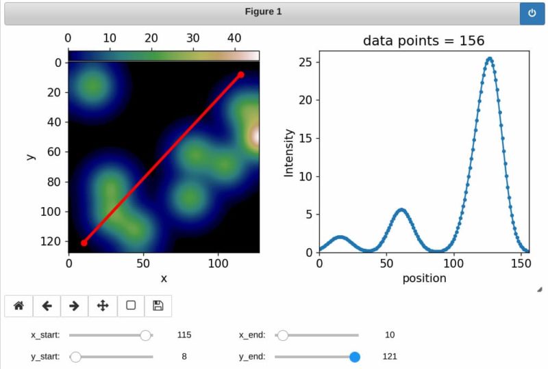
選択した値をset_dataに適用し、画像上にプロファイル取得範囲を点と線で視覚的に表示します。次に、取得した座標をprofile_line関数に渡してプロファイルを抽出し、そのデータもset_dataを使って同様にプロットに表示します。
Widgetsの有効化と表示
interactiveを使って関数fを有効化し、ipywidgetsの動作を実現しました。整理された表示のために、HBoxとVBoxを使ってウィジェットを配置し、display(ui)コマンドで表示しています。
IntSliderを変化させたときの強度プロファイルの変化
参考


Using Interact — Jupyter Widgets 8.1.8 documentation
ipywidgets.readthedocs.io

Widget List — Jupyter Widgets 8.1.8 documentation
ipywidgets.readthedocs.io
コメント