[scikit-image] 22. ハフ変換による楕円の検出(transform.hough_ellipse)

はじめに
コード
解説
参考

はじめに

ここでは、skimage.transform の hough_ellipseを用いた楕円の検出について説明する。

コード

解説

モジュールのインポート

バージョン

画像データの読み込み

rgb2grayでグレースケールに変換する。画像は下記サイトの楕円を採用した。

布のマークのイラスト「矢印・丸・クローバー・スペード・楕円・花・ハート・四角・スペード・星・三角」

いらすとやは季節のイベント・動物・子供などのかわいいイラストが沢山見つかるフリー素材サイトです。

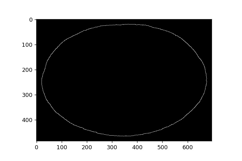
キャニー法によるエッジの検出と表示

canny法でエッジを検出し、ax.imshow(edges, cmap=plt.cm.gray)で表示する。

canny法については、下記で解説した。

[scikit-image] 12. Canny法によるエッジ検出 (feature.canny)

skimage.feature の canny を用いた、Canny法によるエッジ検出

ハフ変換による楕円の検出

hough_ellipse()により、ハフ変換による楕円の検出ができる。

edgesはハフ変換したい画像とする。
accuracyは、精度のことで、短軸方向のaccumulatorのビンサイズとなる。
thresholdはaccumulatorのしきい値で、min_sizeは、楕円の長い方の半径の最小値、max_sizeは楕円の短い方の半径の最大値となっている。
resultをaccumulatorの順にソートして表示している。
結果は、 (‘accumulator’,’yc’, ‘xc’, ‘a’, ‘b’, ‘orientation’)で返ってきて、(yc, xc)は中心の座標、 (a, b)はそれぞれ長軸と短軸のことである。orientationは楕円の向きを示す。

より誤差が少なく近似されている楕円の選出

accumulatorの順にソートしたので最後列のデータが最も誤差が少なく近似されている楕円だと思われる。
結果をリスト形式として、それぞれのデータをスライスで取り出す。

検出した楕円の表示のための準備

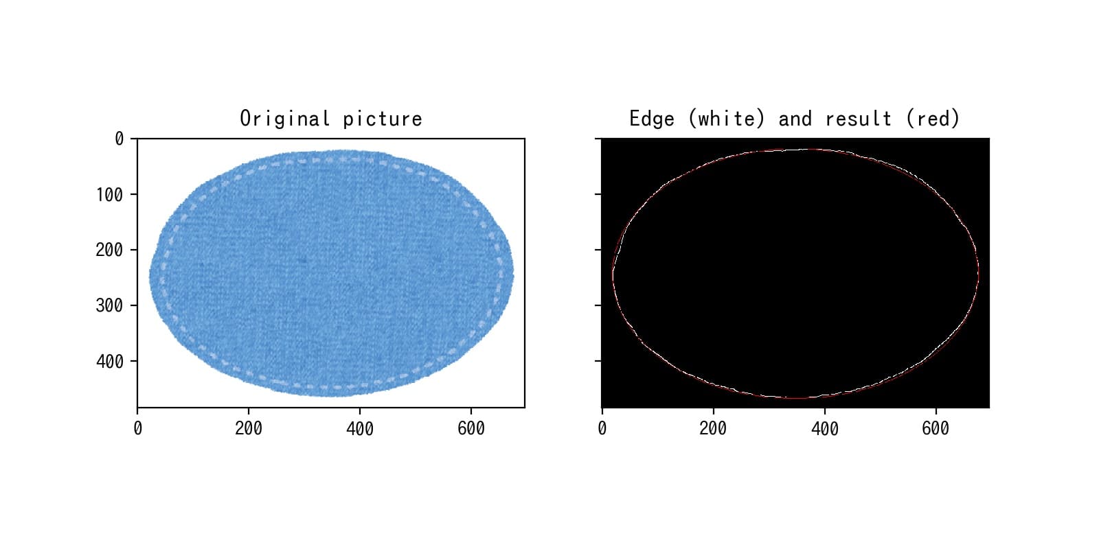
ellipse_perimeter()により画像中に楕円を生成する。座標と各方向の半径、方向を設定することで楕円を生成できる。
生成した楕円に色をつけるために、gray2rgb(img_as_ubyte)により [0〜255]で色を指定できるRGB形式に変換する。
edges[cy, cx] = (250, 0, 0)により、楕円部分のみを赤色にすることができる。

図の表示

コードをダウンロード(.pyファイル)

コードをダウンロード(.ipynbファイル)

参考

Circular and Elliptical Hough Transforms — skimage 0.25.2 documentation

skimage.draw — skimage 0.26.0rc0.dev0 documentation

https://amzn.to/3tgUPhh