[lmfit] 8. フィッティングモデルの信頼区間を表示

はじめに

lmfitは非線形最小二乗法を用いてカーブフィッティングを行うPythonライブラリです。Scipy.optimize.curve_fitの機能を拡張し、より柔軟なパラメータ制約やモデル評価が可能になっています。この記事では、lmfitを使用してフィッティングモデルの信頼区間を表示・評価する方法について詳しく解説します。

信頼区間とは

信頼区間とは、推定されたパラメータが特定の確率（通常95%）で存在する範囲を示すものです。フィッティングの結果得られたパラメータの不確かさを定量化するために重要な指標となります。

コード

解説

モジュールのインポートなど

バージョン

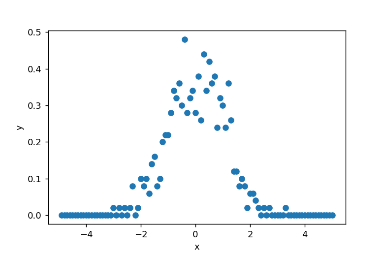
データの生成

np.random.randn(500)を使って標準正規分布に従うデータを500個生成し、np.histgramでヒストグラム化することで正規分布の形状を可視化できます。

図示すると以下のようになります。

初期パラメータの作成

モデルには、定義済みのGaussianModel()を使用します。model.guess(histo, x=bins)によって初期パラメータを自動推定でき、これをフィッティングのパラメータとして利用できます。

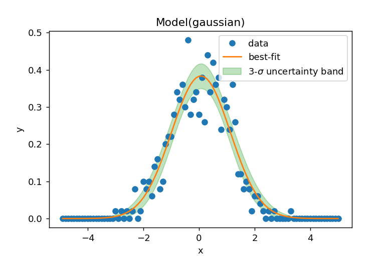
カーブフィットと99%信頼区間

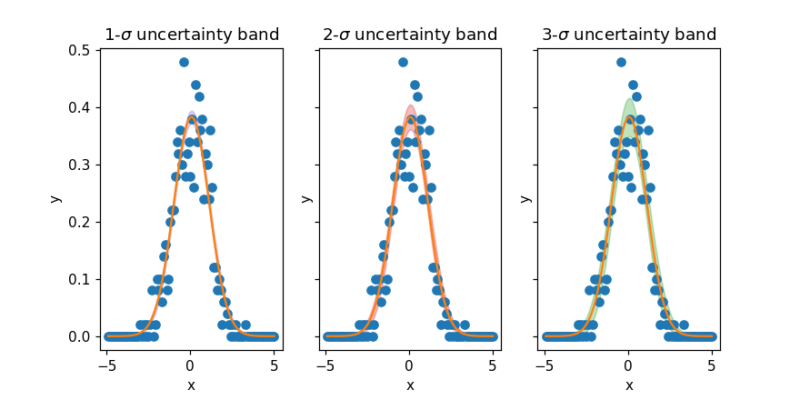
model.fit(histo, params, x=bins)を使用してカーブフィッティングを実行し、result.eval_uncertainty(sigma=3)で99%信頼区間を計算できます。

結果を図示すると以下のようになります。

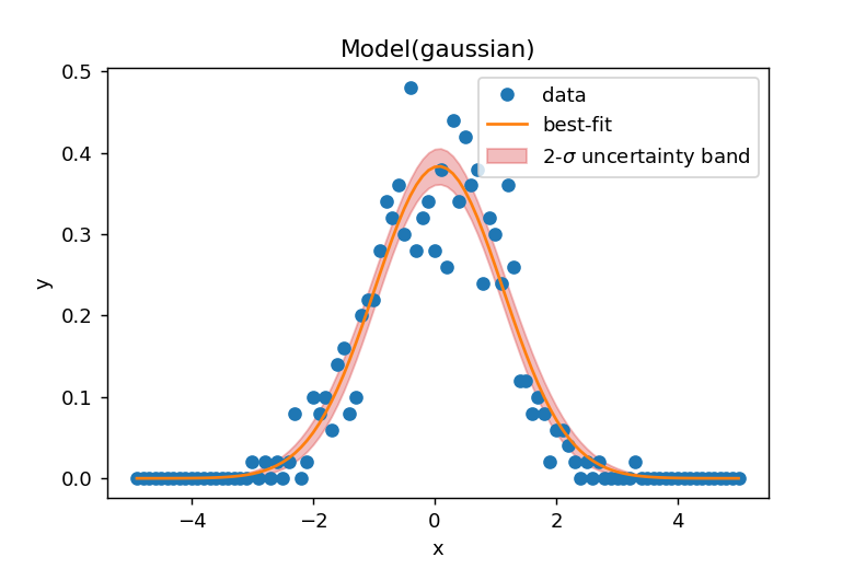
95%信頼区間

95%信頼区間はresult.eval_uncertainty(sigma=2)で計算でき、以下のようなグラフとして表示されます。

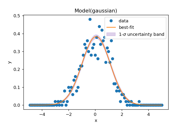
68%信頼区間

68%信頼区間はresult.eval_uncertainty(sigma=1)で計算でき、下図のように表示されます。

subplotsで68–95–99%の信頼区間を並べて表示

コードをダウンロード(.pyファイル)

コードをダウンロード(.ipynbファイル)

参考

Non-Linear Least-Squares Minimization and Curve-Fitting for Python — Non-Linear Least-Squares Minimization and Curve-Fitting for Python

lmfit.github.io

Model - uncertainty — Non-Linear Least-Squares Minimization and Curve-Fitting for Python

lmfit.github.io