[SciPy] 8. np.polyfit, curve_fit, lmfitによる線形近似の実行速度比較

はじめに

np.polyfit, scipy.optimizeのcurve_fit, lmfitによる線形近似の実行速度の比較をmatplotlibのエラーバー付き棒グラフで表示する。

np.arange(0,10,1)で0から9の1刻みの配列を作成して、yのdataにnp.random.rand(10)でばらつきを付与する。

np.polyfit(x,y,1)で1次の式でのフィッティングの係数を求める。具体的にはy=ax+bのaとbがこれでもとまる。
np.polyval(pf,x)で係数pfを使った1次の式のyのdataを生成する。
データと近似式を表示すると下図のようになる。

%timeitで実行時間を計測する。

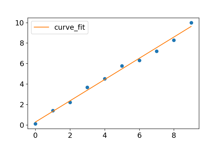
関数を定義して、curve_fitに関数とデータと初期値を渡すことで、係数が求まる。np.polyval(popt,x)で係数poptを使った1次の式のyのdataを生成する。
データと近似式を表示すると下図のようになる。

なお、決定係数の求め方については下記記事で解説した。

%timeitで実行時間を計測する。

lmfitは非線形近似の高レベルなインターフェイスであり、詳細な情報を得ることができる。condaでインストールする場合は、下記のようになる。

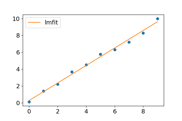
conda install -c conda-forge lmfit

基本的な使い方はcurve_fitと同じであり、modelを定義して、初期値とデータを渡して近似を行う。近似データはresult.best_fitで得ることができる。
データと近似式を表示すると下図のようになる。

%timeitで実行時間を計測する。

polyfitが最速で、curve_fit, lmfitの順で実行時間が長い。